Make a Time Series Forecasting model with BigQuery ML

1. What is Time Series Data?
2. What is ARIMA model?
3. Overview the dataset
4. Prepare the training data
5. Create the ARIMA model
6. Evaluate the model
7. Make a Prediction

What is Time Series Data ?

Time series data is a type of data where observations are collected, recorded, or measured at successive points in time, typically at regular intervals. Time series data can be decomposed into trend, seasonality, cyclicality, and irregularity components. Understanding and modelling these components are essential for accurate forecasting and analysis of time series data.

1. Trend:
   • The long-term movement or directionality of the data over time. It captures the overall tendency of the data to increase, decrease, or remain stable.
   • Trends can be upward (increasing), downward (decreasing), or horizontal (no significant change).
2. Seasonality:
   • The repetitive and predictable patterns that occur at regular intervals within the data, often corresponding to specific time periods such as days, weeks, months, or seasons.
   • Seasonal patterns can be daily, weekly, monthly, quarterly, or annual, depending on the nature of the data and the context.
3. Cyclicality:
   • Similar to seasonality, cyclicality involves repetitive patterns; however, these patterns do not have fixed periods and may occur over longer time spans.
   • Cycles typically represent fluctuations around the trend that are not of fixed frequency or duration.
4. Irregularity (or Residual):
   • The random and unpredictable fluctuations or noise in the data that cannot be attributed to the trend, seasonality, or cyclicality.
   • Irregular components represent the unexplained variation in the data and are often caused by random events, outliers, or measurement errors.

What is ARIMA model ?

ARIMA (AutoRegressive Integrated Moving Average) is a popular statistical method used for time series forecasting. It’s a flexible and powerful approach that can capture a wide range of temporal patterns in data. ARIMA models are especially useful when dealing with non-stationary time series data, where the statistical properties of the series change over time.

ARIMA models consist of three main components:

1. AutoRegressive (AR) Component:
   • The autoregressive component represents the relationship between an observation and a number of lagged observations (i.e., previous time steps).
   • The term “autoregressive” refers to the idea that the value at any given time is linearly related to its own past values.
   • In an AR(p) model, the current value of the time series is modeled as a linear combination of its past p values.
2. Integrated (I) Component:
   • The integrated component refers to the differencing of raw observations (subtracting an observation from its previous observation) in order to make the time series stationary.
   • Stationarity implies that the statistical properties of the time series (such as mean and variance) remain constant over time.
   • The degree of differencing required to make the series stationary determines the “order of integration” (denoted by the ‘d’ parameter). If no differencing is necessary, ‘d’ is set to 0.
3. Moving Average (MA) Component:
   • The moving average component models the relationship between an observation and a residual error from a moving average model applied to lagged observations.
   • Unlike the autoregressive component, which incorporates past values of the series, the moving average component incorporates past forecast errors.
   • In an MA(q) model, the current value of the time series is modeled as a linear combination of past q forecast errors.

Overview the Dataset

SELECT
   bike_id,
   EXTRACT (DATE FROM TIMESTAMP(start_date)) AS start_date,
   start_station_name,
   end_station_name,
FROM
  `bigquery-public-data.london_bicycles.cycle_hire`
  WHERE start_date BETWEEN '2016-01-01' AND '2017-01-01'
  LIMIT 5

Row	bike_id	start_date	start_station_name	end_station_name
1	9546	2016-09-03	St. Martin’s Street, West End	Crosswall, Tower
2	8455	2016-08-31	Hyde Park Corner, Hyde Park	Park Lane, Mayfair
3	12540	2016-08-31	Wardour Street, Soho	Old Quebec Street, Marylebone
4	1801	2016-09-03	George Place Mews, Marylebone	Northdown Street, King’s Cross
5	7890	2016-09-04	Bishop’s Bridge Road West, Bayswater	Jubilee Gardens, South Bank

SELECT
   EXTRACT (DATE FROM TIMESTAMP(start_date)) AS start_date,
   start_station_name,
  COUNT(*) AS total_trips
FROM
  `bigquery-public-data.london_bicycles.cycle_hire`
  WHERE start_date BETWEEN '2016-01-01' AND '2017-01-01'
  GROUP BY
    start_station_name, start_date
LIMIT 5

Row	start_date	start_station_name	total_trips
1	2016-09-05	Bermondsey Street, Bermondsey	66
2	2016-09-03	Exhibition Road Museums, South Kensington	65
3	2016-09-04	Good’s Way, King’s Cross	46
4	2016-09-01	Hammersmith Town Hall, Hammersmith	25
5	2016-09-01	Charles II Street, West End	53

Prepare the training data

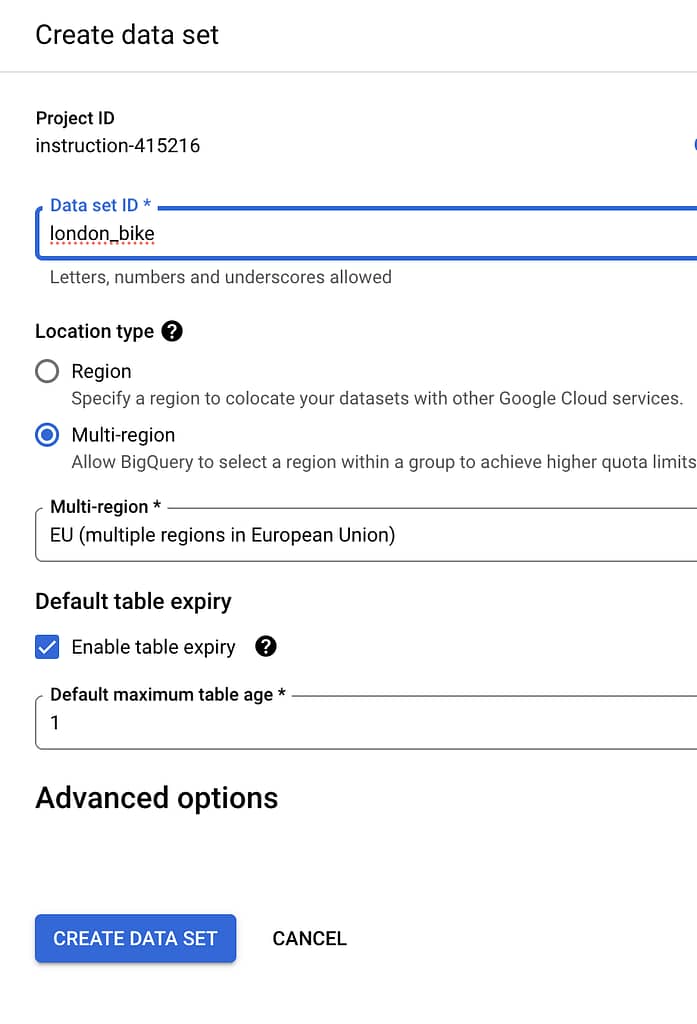
• Create a dataset called ‘london_bike’
• Extract the related data and stored in a table called ‘training_data’

You will see the training data like this

Row	start_date	start_station_name	total_trips
1	2016-05-31	Argyll Road, Kensington	3
2	2016-11-04	Argyll Road, Kensington	4
3	2017-01-01	Argyll Road, Kensington	4
4	2016-03-08	Argyll Road, Kensington	5
5	2016-11-29	Argyll Road, Kensington	5
6	2016-02-05	Argyll Road, Kensington	6

If we group the total trip by each date and visualise it, the graph will look like this:

Create the ARIMA model

CREATE OR REPLACE MODEL london_bike.arima_model
  OPTIONS(
    MODEL_TYPE='ARIMA',
    TIME_SERIES_TIMESTAMP_COL='start_date',
    TIME_SERIES_DATA_COL='total_trips',
    TIME_SERIES_ID_COL='start_station_name'
  ) AS
  SELECT
    start_date,
    start_station_name,
    total_trips
  FROM
    london_bike.training_data

Evaluate the ARIMA model

SELECT
  *
FROM
  ML.EVALUATE(MODEL london_bike.arima_model)

Row	start_station_name	non_seasonal_p	non_seasonal_d	non_seasonal_q	has_drift	log_likelihood	AIC	variance	seasonal_periods
1	Abingdon Villas, Kensington	0	1	5	false	-1056.6241316416781	2125.2482632833562	18.297407336004053	WEEKLY
2	Argyll Road, Kensington	0	1	5	false	-1158.6892923686037	2329.3785847372073	32.014399603264621	WEEKLY
3	Barons Court Station, West Kensington	0	1	5	false	-1210.1825629464847	2432.3651258929694	43.44947290938	WEEKLY
4	Bevington Road West, North Kensington	2	1	3	false	-610.9865111227034	1233.9730222454068	32.723647125570743	WEEKLY
5	Bevington Road, North Kensington	3	1	1	false	-468.18303823240092	946.36607646480184	10.548901269687196	WEEKLY

There are five models trained, one for each of the stations in the training data.

• The first four columns (non_seasonal_{p,d,q} and has_drift) define the ARIMA model.
• The next three metrics (log_likelihood, AIC, and variance) are relevant to the ARIMA model fitting process.

The fitting process determines the best ARIMA model by using the auto.ARIMA algorithm, one for each time series. Of these metrics, AIC is typically the go-to metric to evaluate how well a time series model fits the data while penalising overly complex models.

Make a Prediction

For example, let’s predict the next 15 days trip at a confidence level of 90%

• The horizon defines the number of future time steps for which predictions will be generated.
• The confidence level indicates the level of confidence associated with the predictions.

SELECT * FROM ML.FORECAST(MODEL london_bike.arima_model, 
                  STRUCT(15 AS horizon, 0.9 AS confidence_level))

You will see result like this

start_station_name	forecast_timestamp	forecast_value	standard_error	confidence_level	prediction_interval_lower_bound	prediction_interval_upper_bound	confidence_interval_lower_bound	confidence_interval_upper_bound
Abingdon Villas, Kensington	2017-01-10 00:00:00 UTC	16.937330281401138	6.5208177923359667	0.9	6.2231625318543706	27.651498030947906	6.2231625318543706	27.651498030947906
Argyll Road, Kensington	2017-01-10 00:00:00 UTC	11.031311051787384	7.7366879924962468	0.9	-1.6806179757241146	23.743240079298882	-1.6806179757241146	23.743240079298882
Barons Court Station, West Kensington	2017-01-10 00:00:00 UTC	28.275244623211513	8.4126381947210973	0.9	14.452681302944734	42.097807943478294	14.452681302944734	42.097807943478294
Bevington Road West, North Kensington	2017-01-10 00:00:00 UTC	8.78776709038098	7.9229778417526369	0.9	-4.2302494185682917	21.805783599330251	-4.2302494185682917	21.805783599330251
Bevington Road, North Kensington	2017-01-10 00:00:00 UTC	3.04537238001045	3.7585970023735604	0.9	-3.1302700116086326	9.2210147716295339	-3.1302700116086326	9.221014771

The standard error measures the variability or dispersion of the forecast errors. It indicates the typical deviation of the observed values from the forecasted values. A smaller standard error implies that the forecast is more accurate and reliable.

The prediction interval represents a range within which the true future value is expected to fall with a certain level of confidence. The lower bound and upper bound of the prediction interval define the endpoints of this range.

The confidence interval also represents a range within which the true future value is expected to fall with a certain level of confidence. The lower bound and upper bound of the confidence interval define the endpoints of this range.

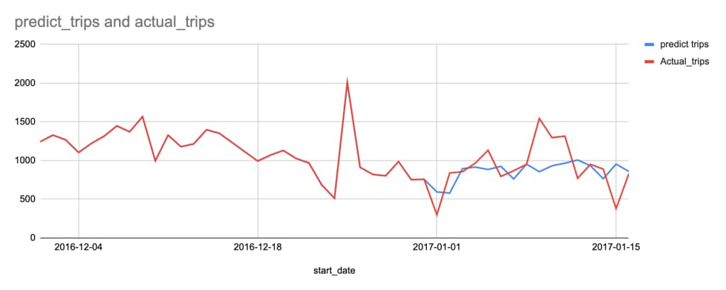
The Predicted Trips and Actual Trips