In this tutorial you will learn how to use Random forest model to make predictions on Iris species.
Dataset
Source: https://raw.githubusercontent.com/mwaskom/seaborn-data/master/iris.csv
The Iris dataset is a well-known and commonly used dataset in the field of machine learning and statistics.It is often used for classification tasks.
The Iris dataset consists of measurements of various features of three species of Iris flowers. Each example in the dataset represents one iris flower, and there are four features (attributes) measured for each flower:
- Sepal Length: Length of the sepal (the green leaf-like structures that protect the flower bud).
- Sepal Width: Width of the sepal.
- Petal Length: Length of the petal (the colorful part of the flower).
- Petal Width: Width of the petal.
Based on these four features, each example in the dataset is labeled with the species of the iris flower it belongs to. There are three species in the dataset:
- Setosa
- Versicolor
- Virginica

Prepare dataset
# import libraries

import matplotlib.pyplot as plt
from pyspark.sql.types import StructType, StructField, DoubleType, StringType
from pyspark.ml.feature import StringIndexer, VectorAssembler
from pyspark.ml.classification import RandomForestClassifier
from pyspark.ml.evaluation import MulticlassClassificationEvaluator
In the snippet below, we first set up a Spark session and then define the schema. But why do we do this?
The type of data we use can greatly affect machine learning outcomes. By outlining the data schema, we make sure that the system loads and understands the data correctly. This helps prevent errors and inconsistencies during processing, making our analysis more reliable and effective.
# create a spark session and load dataset
from pyspark.sql import SparkSession, SQLContext
spark = SparkSession.builder.appName('ML_01_Iris_tutorial').getOrCreate()

# Define the schema
schema = StructType([
    StructField("sepal_length", DoubleType(), True),
    StructField("sepal_width", DoubleType(), True),
    StructField("petal_length", DoubleType(), True),
    StructField("petal_width", DoubleType(), True),
    StructField("species", StringType(), True)
])


# Read the CSV file into a DataFrame
df = spark.read.option('header', 'true').schema(schema).csv(' https://raw.githubusercontent.com/mwaskom/seaborn-data/master/iris.csv')
Process labels and features
In the dataset, the species are Setosa,Versicolor, and Virginica. The data type is string. We need to convert the String data type to numeric. The same thing to the four features:’sepal_length’, ‘sepal_width’, ‘petal_length’, ‘petal_width’. That’s why we use the two functions: StringIndexer() and VectorAssembler()
StringIndexer is used to convert categorical or string-type features into numerical representations. It assigns a unique index to each category in the input column.
VectorAssembler is used to combine multiple columns of features into a single feature vector column.This is useful when you have multiple features that need to be passed as a single input to a machine learning algorithm.
# Encode the 'species' column into numerical labels
indexer = StringIndexer(inputCol="species", outputCol="label")
indexed_df = indexer.fit(df).transform(df)

# Assemble feature vectors
feature_cols = ['sepal_length', 'sepal_width', 'petal_length', 'petal_width']
assembler = VectorAssembler(inputCols=feature_cols, outputCol='features')
final_df = assembler.transform(indexed_df)
final_df.show()
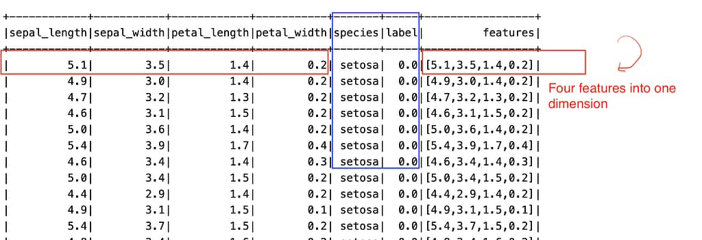
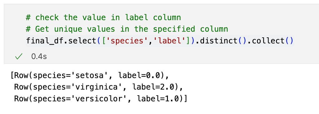
As we can see from the two images, the species have been transformed into numerical labels.
The four features habe been converted into one dimensional column called features.
Train model
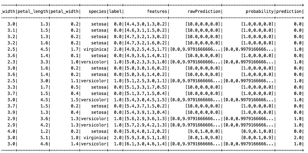
# Split the data into training and testing sets
train_data, test_data = final_df.randomSplit([0.8, 0.2], seed=2024)

# Step 3: Train a model
rf = RandomForestClassifier(labelCol='label', featuresCol='features', numTrees=10)
model = rf.fit(train_data)

# Step 4: apply the model
predictions = model.transform(test_data)
predictions.show()
Evaluate Model
# evaluate the model
evaluator = MulticlassClassificationEvaluator(labelCol='label', predictionCol='prediction', metricName='accuracy')
accuracy = evaluator.evaluate(predictions)
precision = evaluator.evaluate(predictions, {evaluator.metricName: "weightedPrecision"})
recall = evaluator.evaluate(predictions, {evaluator.metricName: "weightedRecall"})
f1_score = evaluator.evaluate(predictions, {evaluator.metricName: "f1"})

print("Accuracy:", accuracy)
print("Precision:", precision)
print("Recall:", recall)
print("F1 Score:", f1_score)
-----------------------------------------------------------
Accuracy: 0.9411764705882353
Precision: 0.9518716577540107
Recall: 0.9411764705882353
F1 Score: 0.9416666666666667
In summary, accuracy measures overall correctness, precision measures the quality of positive predictions, recall measures the ability to capture all positive instances, and F1-score provides a balance between precision and recall. These metrics together provide a comprehensive assessment of the model’s performance in multi-class classification tasks.